Colebrook Equation

Overview

The Colebrook equation (also known as the Colebrook–White equation) is the standard implicit relationship for calculating the Darcy–Weisbach friction factor in turbulent pipe and duct flow. It accounts for both viscous effects (via the Reynolds number) and surface roughness, bridging the smooth-pipe and fully-rough regimes described on the Moody diagram.

Because the friction factor appears on both sides of the equation, it cannot be solved algebraically and requires numerical iteration.

Friction loss coefficients in pipes, tubes and ducts.

Key Formulas

Colebrook Equation (implicit)

$\frac{1}{\sqrt{f}} = -2\,\log_{10}\!\left(\frac{\varepsilon/D}{3.7} + \frac{2.51}{Re\,\sqrt{f}}\right)$

Swamee–Jain Explicit Approximation

An explicit approximation valid for $5\,000 \le Re \le 10^8$ and $10^{-6} \le \varepsilon/D \le 10^{-2}$:

$f = \frac{0.25}{\left[\log_{10}\!\left(\dfrac{\varepsilon/D}{3.7} + \dfrac{5.74}{Re^{0.9}}\right)\right]^2}$

This form is useful for spreadsheet calculations and programming when iterative solvers are not available.

Pressure Drop (Darcy–Weisbach)

Once $f$ is known, the major head loss is:

$h_f = f\,\frac{L}{D}\,\frac{v^2}{2\,g}$

Variables

Typical Pipe Roughness Values

Friction Factor vs Reynolds Number

The chart below uses the Swamee–Jain approximation to show how the friction factor varies with Reynolds number for three relative roughness levels.

Unit Converter

Restored Original Source Tables

The following tables are restored from the original source page to preserve the complete reference data.

The cached source page also contains a non-engineering layout/search table. For strict source-table preservation, the detected rows are reproduced below and are not friction-factor data.

Original Source Images

The following original source images are preserved to avoid losing visual reference material. When an image contains chart or tabular data, its extracted values are represented in the page tables, calculators, or interactive charts; remaining images are retained as visual source references.

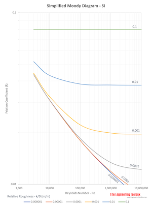
The Moody diagram chart images are represented interactively above by the Darcy friction-factor curve chart generated from the Swamee-Jain approximation. The static source images are retained below as visual references.

Moody diagram SI

Engineering Notes

• Turbulent flow only. The Colebrook equation is valid only in the turbulent regime ($Re \gtrsim 4\,000$). For laminar flow ($Re < 2\,300$), use $f = 64/Re$.
• Friction coefficient at laminar flow. The original source note is preserved here: for fully laminar pipe flow the friction coefficient is calculated directly as $\lambda = 64/Re$.
• Iteration required. Because $f$ appears on both sides, a direct solution is not possible. Common numerical approaches include the Newton–Raphson method, fixed-point iteration, or the Swamee–Jain approximation shown above.
• Transition zone caution. In the transition-roughness region ($2\,300 < Re < 4\,000$), flow regime is uncertain and friction-factor predictions carry higher uncertainty.
• Hydraulic diameter for non-circular ducts. When applied to rectangular or non-circular cross-sections, replace $D$ with the hydraulic diameter $D_h = 4A/P$, where $A$ is the flow area and $P$ is the wetted perimeter.
• Roughness aging. The roughness values in the table above represent new/clean conditions. Over time, corrosion, scaling, and biofouling can significantly increase $\varepsilon$, raising the friction factor and pressure drop. Design with a roughness value one category higher than the new-pipe condition is common practice.
• Moody diagram alternative. The friction factor can also be read graphically from the Moody diagram, which plots $f$ against $Re$ for lines of constant relative roughness $\varepsilon/D$.

References

• Colebrook Equation — Engineering ToolBox